
success on their ability to manage returns. But nobody really manages returns.
The only thing advisors can do is manage wealth, and once you and your clients
understand that simple but enormous distinction, you’ll both be wealthier for
it.
measurable what cannot be measured.”
There is an old saying that “you cannot manage what you do not measure.” A
lot of effort in the investment consulting and financial advising industry
involves measurement, specifically performance measurement. Track records of
funds and money managers are measured and benchmarked using indexes or ranked
among supposed peers. Many financial advisors represent to their clients that
part of their ongoing value is regularly measuring account performance.
But is measuring returns the same as managing results?
I personally think the old saying should be appended with this statement:
“But just because you measure something does not mean you are managing it.”
Sophistication in investment performance measurement has advanced remarkably
over the last several decades with custom benchmarking, dollar- and
time-weighted return calculations, and even online daily reporting. The
financial services industry is clearly measuring a lot of returns, but does
doing so add any value?
Is the measurement of returns leaving investors with a potentially false and
misleading impression that those returns are also being managed, merely because
they are measured? Is it even possible to manage returns? If so, what would
successful management mean to the end investor, and how would one manage it?
What are we measuring?
Which returns are we attempting to manage? Are we measuring and managing
time-weighted returns (those that ignore cash flows and wealth results)—or
dollar-weighted returns (those tied to wealth results)? There is a massive
difference. Most in the financial services industry claim they manage and
measure both time- and dollar-weighted results. Advertisements profess a
tradition of a “disciplined approach” with “vast resources of a global
organization” to control risk, produce superior returns, or even do both,
measured on a time-weighted market-relative basis. Such results are often used
to justify the cost of their “wealth management” services.
But are superior time-weighted, risk-adjusted returns of any value to the
investor? One would think so, considering the effort being spent measuring,
reporting, and selecting investment alternatives to produce superior
time-weighted returns. But if obtaining successful risk-adjusted returns on a
time-weighted basis doesn’t necessarily produce more wealth, what good is the
ability to manage it? Is it all just an optical illusion or a marketing sleight
of hand?
The premise behind attempting to produce superior time-weighted returns often
completely ignores the risk of materially underperforming that is
introduced—risk one can almost certainly avoid by indexing.
Finally, how long a time frame is needed for the evidence supposedly provided
by the measurement of returns to draw an objective valid conclusion of “success”
(instead of randomness)? If successful management is evidenced in the results,
is the period long enough to avoid being skewed by one data point, or the random
timing thereof that might occur? In essence, is 10 years of “success” truly
successful if the results were merely caused by timing of one or two years when
the superior market-relative returns occurred?
Testing premises
To test whether there is real wealth value in the ability to produce superior
time-weighted returns (risk-adjusted) over the long term, we need to examine the
ultimate effect on real investor scenarios so we can see the wealth impact on a
dollar- or wealth-weighted basis. We also have to eliminate the extreme random
noise that often occurs with improper benchmarking or extreme deviations from
the allocation policy. Extreme random noise could excessively skew the results
and would be misleading—a legal and ethical violation.
We would also need to observe the effect in both dollars and time-weighted
returns of fairly small changes to the timing of just one or two data points.
This is necessary to test the validity of whether 10 years of data is merely the
effect of when one or two years of superior or inferior market-relative results
occur.
The scenarios used will contrast three investors to test these effects and
the ultimate dollar benefit or cost of the supposed value of “successfully”
managing “superior” risk-adjusted returns.
- The neutral model. Our first investor is represented by the
typical growth of $100, as is often used in examining time-weighted returns that
will always precisely match the compound return. This, of course, is a result
that assumes the investor is neither contributing to nor withdrawing money from
the portfolio over the entire time horizon. Judge for yourself how many
investors neither save nor spend money. - The spender. The second investor is a more realistic example
of a spender and represents someone who is using his portfolio to support his
lifestyle. For the spender example, presume you have an investor that sold his
company stock for $1 million after tax at age 60 and now wishes to retire. He
would be very comfortable with a retirement income spending goal of $100,000 a
year adjusted for inflation.While a $100,000 annual after-tax spending need is obviously more than could
be sustained from a $1 million portfolio, he fortunately has a pension, a
401(k), and Social Security, which will provide him with sufficient sources of
income so long as he chooses to delay receiving those benefits until age 70.
Therefore, he can easily spend both investment returns and principal from his $1
million portfolio for the next 10 years until such time that he elects to take
his pension and Social Security and is forced to make withdrawals from his
401(k) at 72½. - The saver. The saver is our third sample investor. She has
only accumulated $100,000 so far, but she just recently received a major
promotion that will enable her to save $100,000 a year after tax for the next 10
years, at which point she wishes to retire. Her goal is to maximize the amount
accumulated over the next 10 years to fund her retirement. She is willing to
adjust her lifestyle at retirement based on how much she accumulates over the
next 10 years. She is also eligible to receive Social Security benefits, which
will buffer some of the uncertainty about her future retirement lifestyle.
Measuring the wealth effect
In measuring the wealth benefit of producing long-term superior time-weighted
returns, we will contrast a fictitious “Manager A” and “Manager B” to a
theoretical benchmark-indexed allocation. The returns used will be net of all
expenses, including the indexed alternative. Both managers never vary from the
benchmark allocation return by more than 6% in any year, and their correlation
coefficient and r-squared are very high relative to the benchmark allocation. In
bear markets, both managers control risk better than the benchmark, and their
return over the 10-year period, net of expenses, exceeds the benchmark by 0.50%
on average. Less risk and more return—the value so many advisors and managers
sell.
In Table 1, we see an example of two such theoretical managers and a sample
of how the theoretical benchmark allocation might behave in any random 10-year
period, along with the ending wealth results for the growth of $100, our
spender, and our saver.
| Table 1: Theoretical Managers and Benchmark Results |
 |
The higher return and lower risk of the managers for the neutral,
growth-of-$100 investor matches the time-weighted returns perfectly to the
average return and risk (and thus, in combination, the geometric mean or
compound return). Manager A and Manager B both grow to more than $222 for this
investor who is neither saving nor spending, with the indexed benchmark coming
in about $11 shy of the managers on the initial $100 investment.
Great results with less money
Despite the time-weighted “superior” risk-adjusted returns of the managers,
the wealth result obtained for our spender with Manager B actually ended up
costing him $63,000 relative to the lower-return and higher-risk indexed
benchmark. Comparing Manager B relative to Manager A (that was practically
identical based on time-weighted measurements) cost the spender nearly 50% of
the ending portfolio value. Manager A beats Manager B, but benchmark beats
Manager B even with “inferior” risk-adjusted returns.
Pick A or B to win or lose
The reverse is true for the managers’ superior time-weighted returns for our
saver, with Manager B producing almost $200,000 more wealth than Manager A and
falling short of the indexed benchmark by nearly $30,000, again despite the
lower returns and higher risk of the benchmark. Manager B beats Manager A, but
benchmark beats Manager A.
Shouldn’t this raise some questions? In this little example, we are
completely ignoring the potential risk introduced—which is substantial—of
materially underperforming the benchmark result, a risk that is almost certainly
avoidable by indexing over the entire time frame. Both Managers A and B produced
better time-weighted, risk-adjusted returns. But whether such “better”
time-weighted returns really produce more wealth is completely uncertain and
unique to the individual’s wealth management goals.
What would it take to truly manage and deliver on the superior wealth
management claim if the means of producing the superior wealth result is based
on the attempt to produce superior risk-adjusted returns? For the management of
wealth, advisors would not only need to be able to select superior management on
the basis of time-weighted returns (not the easiest task), but also, they would
need to know when superior results would occur in the future based on the unique
investor’s wealth management plan.
To add value—at least, in dollars instead of potentially meaningless
time-weighted risk-adjusted returns—they would have to know that most of the
superior performance of Manager B will occur in the later years, making it a
better choice for the saver who will have more wealth accumulated when the
superior results occur. Or, that for our spender, the superior results of
Manager A will be concentrated toward the beginning of the 10-year period before
withdrawals have depleted some of the capital.
Some advisors claim they can time both, since it would be best to have
Manager A for the first six years and then after six years of massively superior
results, they would switch to the underperforming Manager B to capture the
turnaround. I’ve yet to see advisors consistently deliver on this promise. Do
they regularly recommend replacing massively winning managers in favor of poorer
managers? More often than not, what I’ve observed is the reverse, replacing the
inferior Manager B years after his results have faltered in favor of a
supposedly better Manager A—resulting in capturing the worst of both managers.
“When” matters to both time- and dollar-weighted results
Many advisors understand that dollar-weighted returns (and thus wealth) are
sensitive to this timing uncertainty of returns when there are contributions and
withdrawals involved. After all, returns can be reordered in any way and the
result for the growth of $100 will be identical, as will the compound return.
Sort the returns from highest to lowest, or lowest to highest, and the answer
will remain unchanged. The standard deviation will not change either merely
because the returns were reordered. One thing will change that is usually
ignored: the market-relative return in each of the individual years, and
therefore also the correlation and r-squared.
Take Manager A from Table 1 and look at the difference in returns from the
market benchmark in each individual year as shown in Table 2, where we examine
the difference relative to the market in each individual year and the statistics
that change and remain unchanged when the order of returns are changed.
| Table 2: Changing the Order of Returns |
 |
When the returns of Manager A are ordered from low to high, we observe that
indeed the compound return, the average return, the standard deviation, and
growth of $100 all are unchanged, as would be expected. However, the difference
from the market in each individual year explodes to as much as a 33% difference
in the first year. This causes both the correlation and r-squared to drastically
decline.
There is obviously a misconception about “long-term,” time-weighted,
risk-adjusted returns being unaffected by the ordering of returns. It would
obviously be evidence of some huge market-relative gambles if a manager deviated
from the benchmark so violently as indicated by Manager A’s returns, ordered
from lowest to highest. Underperforming by 33% in one year and then
outperforming by 25% and 21%, respectively, in two other years could only be
accomplished with wild bets against the asset-class benchmark.
Of course, this is an extreme example to emphasize the point. But the key
thing to understand here is that the assumption so many investors and advisors
make about long-term, risk-adjusted returns relative to the market is that such
returns are not really relative to the market. In essence, long-term,
time-weighted returns and dollar-weighted results are both affected when just
one or two years of superior or inferior market-relative returns occur.
A simple example of this effect can be observed by examining whether those
statistics (i.e., compound and average return, standard deviation, and growth of
$100) that are unaffected by reordering the manager’s returns also remain intact
when we reorder the market-relative return. Table 3 shows the market benchmark
returns and the original order of the returns for Manager A, and then
demonstrates what happens if one merely swaps the two years for the most extreme
market-relative returns. We find that swapping two years relative to the market
changes the statistics that normally do not change when returns are
reordered.
| Table 3: Swapping Years (shaded areas are unchanged from Table 1) |
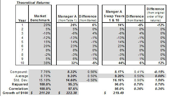 |
The results in Table 3 demonstrate that time-weighted risk-adjusted returns
can be dramatically impacted by just one or two years of market-relative
returns. Outperforming the market by 6% in the 10th year and underperforming the
first year (rather than the reverse) lowered the compound return and the growth
of $100. Swapping the timing of the most extreme market-relative performance
caused the standard deviation to change by 1.56 points from being 0.58% less
than the benchmark to being 0.98% more than the benchmark!
While the average return remained unchanged, the r-squared and correlation
increased. In fact, other than the average return remaining the same, all those
statistics that normally do not change when returns are reordered indeed do
change because of the timing when the superior and inferior market-relative
returns occurred.
What does this mean to managing wealth? What does this mean about managing
returns? One must acknowledge that over the long term, superior (or inferior)
risk-adjusted returns can be caused by what is, in essence, the timing of
market-relative alpha. If the timing of superior and inferior market-relative
results impacts the growth of $100, what would happen with our saver and spender
cases?
To test the wealth sensitivity to this truly market-relative alpha timing, I
swapped the years in which the best and worst market-relative returns of both
Managers A and B occurred. In so doing, we can observe the wealth effect for all
of our sample investors as well as the impact of the time- and dollar-weighted
results as shown in Table 4.
| Table 4: Swapping the Best and Worst Market-Relative Results (shaded areas are unchanged from Table 1) |
 |
This small change in only two years of market-relative results—not affecting
the 10-year average return—has a big impact. First, the results for the neutral,
growth-of-$100 investor declined for both managers because their standard
deviation increased to be above the market benchmark, whereas before the swap,
the risk was below the benchmark. So much for the timing of returns not
impacting a portfolio in the absence of cash flows! On a market-relative basis,
it certainly can impact the risk, compound return, and wealth. This was based on
just swapping the years that the most extreme market-relative performance
occurred (years 1 and 10 for Manager A, and years 1 and 9 for Manager B).
This means that even for time-weighted returns, relative to the benchmark,
the timing of one or two years can create a false perception of time-weighted
value, despite the full 10-year observation period. We also notice that the best
results for our spender and saver investors have swapped managers. The choice of
the optimal manager similarly hinges on timing which years produce superior or
inferior market-relative returns.
Lastly, the best result among the choices has declined for both the saver and
spender.
Measuring temperature with a ruler
When success is being measured in these return-based measures, which may not
necessarily equate to anything other than random one- or two-year observations,
it’s like attempting to measure the temperature of one’s wealth with a ruler.
All of this return measurement produces nothing more than misleading
information. Can we really control both how much and when superior results will
occur, since doing so is necessary to truly manage any investor’s wealth?
Randomness is random
Monte Carlo simulations have been adopted by many in the industry to deal
with the timing effect of returns on wealth management plans—often at the
expense of the investor’s lifestyle, by attempting to get to the highest “odds
of excess” (frequently misstated as “odds of success”). For example, when
simulations are run for a set of life goals, many advisors tell clients that
they have a 90% chance of success, but 95% would be better. This makes it sound
as though it were a simple pass/fail grade.
But what 90% confidence means (with well-thought-out capital market
assumptions) is that there were 900 of 1,000 simulations that met all of the
client’s goals and exceeded the estate goal. Perhaps 800 of the 1,000 trials
doubled or tripled the estate goal. Regardless of how Monte Carlo simulations
are misused, the question still remains about measuring the uncertainty of the
timing of returns. Is measuring the timing of return uncertainty the same thing
as managing it?
It is possible to manage wealth, but you won’t be able to do it if you are
attempting to manage returns, as the examples in this article have demonstrated.
Managing wealth is much different from managing returns. The process used to
manage defined-benefit pension plans is a good example of true wealth
management. Managing a defined-benefit plan is mathematically similar to wealth
management for an investor. Both have contributions (savings), liabilities
(spending or estate goals), current portfolio values, asset allocation policies,
and so on.
But pensions also measure their funded status and consider the choices of all
of these variables together—and they manage the choices across all these
variables. When pensions are overfunded, choices are considered to reduce
investment risk, increase benefits, reduce future contributions, or even
terminate the plan to recapture the excess funding.
Why shouldn’t individual investors be offered the same management choices?
When pensions are underfunded, the investment policy risk exposure may be
increased, benefits reduced, or contributions increased. Shouldn’t an
individual’s wealth management plan be handled in the same way?
Doing so takes a complete rethinking of traditional investment consulting and
financial advising. The dramatic effects in the 10-year examples outlined in
this article—and even the impact of just one year on those results—apply over
the long term of 80 years as well. Managing the wrong thing is not really
providing value, no matter how much you measure it.
You cannot manage everything you can measure. But you can manage wealth
instead of returns.
